In the first version of this project, I used a logistic regression model on EEG-derived features. It technically worked, but in practice it was frustrating to use live. Tuning thresholds during a demo was hard, the behavior felt opaque, and performance drifted noticeably from one session to the next. In this version, I moved to a fully on-device, rule-based pipeline that is easier to understand, easier to debug, and easier to tune in real time.
This writeup is beginner-friendly. It explains what EEG and EOG are, where to place electrodes for a simple Fp1/Fp2-style setup, what the FFT is doing conceptually, how the Arduino decides focus and blink events, and how the macOS app controls the system in real time.
You can follow this with the code on Github: https://github.com/Montekkundan/mindclick
The goal is to produce three reliable control signals, all emitted as real-time keyboard outputs so they can drive games, editors, or general app controls:
Focus trigger
Double blink trigger
Triple blink trigger
In this build, the system is single-channel, so EEG is best used as one coarse state signal rather than multiple independent commands. With only one channel, different mental commands are hard to separate robustly in real time, and they drift a lot with placement and session noise. That is why this design uses EEG only for a single focus state, and uses EOG for discrete commands.
If this were a multi-channel system (more electrodes and spatial information), you could realistically add richer control signals, such as multiple EEG-based states or better separation of different intention patterns. With more channels, you have more degrees of freedom and better signal discrimination, which makes multi-command EEG more feasible.
EEG vs EOG
EEG (electroencephalography) is the measurement of tiny voltage fluctuations from the scalp that are related, indirectly, to brain activity. EOG (electrooculography) is the measurement of voltage changes caused by eye movement and blinks. Both are “electrical signals,” but they behave very differently.
For a practical DIY control system, each signal type has a sweet spot. EEG is better suited for estimating broad, slow-changing state, such as whether you are “more focused” or “less focused.” EOG is much better suited for discrete commands, because blinks are strong, obvious events that stand out clearly compared to most other activity.
That leads to a simple, robust design split:
EEG → focus state
EOG → blink commands
Keeping these paths separate makes the system easier to tune and prevents one type of detection logic from interfering with the other.
Hardware and software stack
The overall system is intentionally simple:
The EEG front-end is a BioAmp EXG-style single-channel analog front-end.
The microcontroller is an Arduino UNO R4 Minima.
The firmware lives in control/control.ino.
The desktop operator interface is a SwiftUI macOS app in thought/.
The Arduino and the app communicate over USB serial using a line-based protocol.
One important behavior is that detection starts OFF by default at boot. The firmware will not begin event detection until it receives an explicit command to enable it. This makes demos safer and prevents accidental triggers on startup.
Electrode placement (Fp1/Fp2-style setup)
This build uses a practical three-electrode placement that is quick to set up and repeat across sessions.
The wiring is:
IN+ (active) goes on the forehead, roughly between the Fp1 and Fp2 region.
IN- goes behind one earlobe, on a bony area.
REF goes behind the other earlobe.
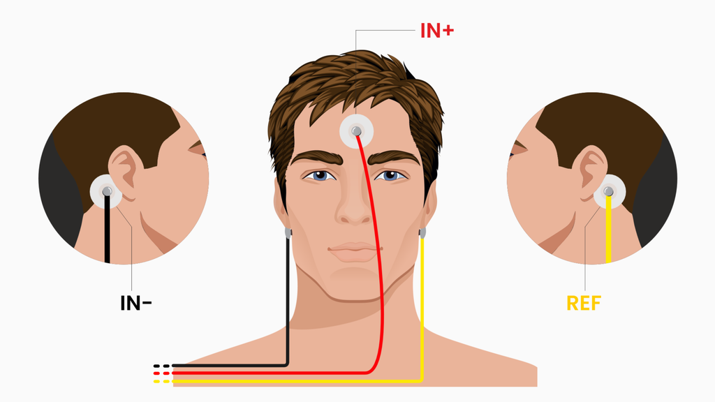
This placement is useful because the forehead is an accessible frontal location that captures a mix of frontal EEG activity and ocular influence, while the earlobes provide convenient, relatively low-muscle reference points. It is not perfect, but it is realistic for DIY and gives repeatable behavior if you keep the setup consistent.
A few practical tips matter more than people expect. Clean the skin before placing electrodes. Keep contact pressure stable during use. If the signal suddenly changes a lot, reseat the electrodes, because that often means the contact impedance changed.
What the FFT is doing and why it helps
The Arduino receives samples in the time domain, meaning it sees voltage values changing over time. Raw time-domain EEG is noisy and difficult to interpret directly, especially if your goal is something like focus.
An FFT (Fast Fourier Transform) converts a short window of time-domain samples into a frequency-domain representation. Instead of asking what is the waveform doing, you can ask how much energy is present in certain frequency ranges. For focus estimation, that frequency-domain view is much easier to work with.
In the current firmware:
The sample rate is 512 Hz.
The FFT size is 512 samples.
The firmware computes a power spectrum and integrates it into bandpower buckets (delta, theta, alpha, beta, gamma).
From these buckets, it derives a smoothed beta percentage.
The key idea is that instead of reading unstable raw EEG values, the system reads a more stable feature: a beta power ratio that can be smoothed and thresholded.
Arduino signal pipeline
The firmware runs two mostly independent pipelines: one for EEG-based focus state and one for EOG-based blink commands.
EEG path (focus)
The EEG path starts with filtering, because real signals contain mains interference, movement artifacts, and other noise. The firmware applies a notch filter to suppress mains noise, then applies an EEG filter suitable for the bandpower workflow.
Next, the firmware runs the FFT, builds the power spectrum, and integrates power into frequency bands. From these, it computes a smoothed beta percentage.
Finally, the firmware uses a focus state machine rather than a single threshold. This makes the output behave better in real time. It uses:
A focus enter threshold (beta) and a focus exit threshold (beta_off) to create hysteresis.
Vote gating, meaning focus must be consistently above or below threshold for a number of consecutive windows.
A minimum ON time to prevent rapid flicker.
A re-entry debounce to avoid immediate re-triggering.
This is what makes the focus trigger feel stable instead of jittery.
EOG path (blinks)
The EOG path is designed for discrete commands. It starts with an EOG filter to emphasize blink-like events. Then it computes an envelope using a moving average over the absolute value of the signal. That turns blink spikes into a smoother activity trace.
A blink is detected when the envelope falls within a tuned threshold window (from blink_low to blink_high). After detecting individual blinks, the firmware groups them in time to detect patterns:
Two blinks in a short window produce a double blink event.
Three blinks in a short window produce a triple blink event.
Because blink events are strong and discrete, this path tends to be much more reliable for command triggering than trying to use EEG alone.
Why I moved away from logistic regression
The earlier approach used logistic regression over extracted features. While it worked, the live behavior did not feel transparent. Small differences in signal quality, electrode placement, or session conditions could shift the model confidence enough that tuning became unpredictable.
There was also a practical data issue. Logistic regression still needs a meaningful amount of labeled data per session and per user to be reliable, especially when the output is discrete click-like triggers. Since I am working alone, I could not realistically collect enough high-quality labeled data across many sessions to make the classifier stable and accurate for real-time command output.
The current approach uses deterministic rules, calibration, and runtime tuning. The biggest advantage is debuggability: you can see exactly which threshold or state transition caused a trigger. It also reduces operational complexity because everything runs on the Arduino without depending on a learned model.
The tradeoff is that rules are less adaptive than a learned model, but for this hardware class and this real-time use case, controllability matters more.
Serial protocol
The macOS app and the Arduino communicate using line-based commands over USB serial. The protocol exists so the system can be tuned and controlled live without reflashing firmware.
Core commands include enabling detection, requesting the current configuration, triggering test events, and setting thresholds and timing parameters.
For example:
enable on
set beta=1.45
set beta_off=1.15
set focus_on_votes=4
set focus_off_votes=3
set focus_min_on=900
set blink_low=30
set blink_high=45
get config
The important design point is that both the Serial Monitor and the macOS app use the same protocol. The app is not doing secret extra logic. It is simply a better interface for sending commands, visualizing values, and managing key mappings.
What the macOS app does
The desktop app acts like a native control console for the firmware. It handles connecting and disconnecting from USB serial, toggling detection ON or OFF, and showing live values such as beta percentage, thresholds, and blink window behavior.
It also provides quality indicators (signal quality and calibration quality), starts calibration flows, and lets you define global or per-app keybind overrides. It includes a way to trigger test events and show toast-style feedback so you can verify the end-to-end pipeline.
The key architectural decision is that heavy DSP stays on the Arduino. The app focuses on runtime control and visualization.
Calibration flow (and why quality can be poor)
Calibration is split into phases:
Relax
Focus
Blink
During calibration, the firmware computes suggested thresholds for focus and blink detection and reports both the suggested values and an overall calibration quality rating (good or poor).
It is important to understand that signal quality and calibration quality are not the same thing. Signal quality mostly reflects whether electrode contact and noise levels are stable. Calibration quality reflects whether the relax and focus conditions were meaningfully separable.
So you can have good contact but poor calibration if, for example, you move your eyes or jaw a lot during relax and focus. Those artifacts can blur the difference between states even when the signal is clean.
Known limitations
This is a DIY, single-channel prototype, and it should be framed that way. Focus is not a perfectly separable binary state. Motion artifacts can still appear. Session drift is real. False positives and false negatives can happen.
Demo checklist
Before a demo, the workflow looks like this. Place electrodes carefully (forehead for IN+, earlobes for IN- and REF). Connect the Arduino and open the app. Verify the serial connection. Enable detection. Run calibration once.
After that, check three things: signal quality, calibration quality, and whether live beta behavior makes sense relative to the thresholds. Then test double and triple blink key outputs in the target application.
If focus feels too jumpy, increase focus_on_votes, increase focus_debounce, or raise beta slightly. If focus feels too sticky, reduce focus_off_votes or raise beta_off slightly.
Final takeaway
Version 1 proved the idea was feasible. Version 2 made it usable by moving everything important into an on-device pipeline, separating EEG state from EOG commands, using robust state logic, exposing runtime control over serial, and adding a native macOS interface for live operation.
Post of 2025-11-16 version 1
TLDR
Hardware: BioAmp EXG Pill, Arduino, Ag/AgCl electrodes, laptop.
Montage: Active at C3, reference at right mastoid or earlobe, ground on forehead.
Processing: Bandpass 5 to 40 Hz, notch 60 Hz, Welch power spectral density.
Features: Alpha 8 to 12 Hz, Beta 13 to 30 Hz, and the Beta to Alpha ratio.
Classifier: Logistic regression with a short calibration session to set a probability threshold.
Outcome: Robust online control with a 0.6 s decision window and refractory to limit false positives.
Demo
Safety and Responsibility
Unless medically indicated, BCI work is exploratory and should avoid any implied therapeutic claims. Use fresh electrodes, clean skin, avoid mains noise and never connect yourself directly to powered circuits without galvanic isolation.
Bill of Materials
BioAmp EXG Pill with shielded leads and gel electrodes
Arduino or compatible microcontroller with serial streaming
USB isolation if available
Headband or cap to hold the C3 electrode
Laptop with Python 3
I used DIY Neuroscience Kit – Pro which has all the materials. You can checkout upsidedownlabs store for cheap materials!
Electrode Placement
Before we talk about rhythms, it helps to be clear about where on the head we are listening from.
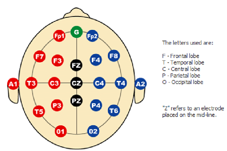
In EEG we use a coordinate system called the international 10-20 system [1-3]. It was introduced in the 1950s as a standardized way to place electrodes so that laboratories in different countries were all talking about the same spots on the scalp [1-3]. The numbers 10 and 20 refer to the fact that the distances between neighboring electrodes are either 10 percent or 20 percent of the total front to back or left to right distance of the head [3].
The letters tell you the lobe that sits underneath
F for frontal
C for central or sensorimotor
P for parietal
O for occipital
T for temporal
The odd numbers (1, 3, 5, 7) are on the left side, and the even numbers (2, 4, 6, 8) are on the right side, with Z meaning the midline. So C3 literally means the central region, left hemisphere, at a standard distance from the midline.
When I first learned this system it felt like a random grid of letters and numbers. What made it click for me was realizing that C3 is not a magic point, it is simply a reproducible way to say “slightly left of the top of the head, above the hand area of the sensorimotor cortex”. If you and I both place an electrode at C3 using the 10-20 rules, we are roughly sampling from the same patch of cortex.
For this project
Place the active electrode at C3 according to the 10-20 system. For right hand imagery C3 is often the most informative single site because the left sensorimotor cortex controls the right hand.
Place the reference on the contralateral mastoid or earlobe to reduce common noise between the two electrodes.
Place ground on the forehead or Fpz.
Check impedances and ensure stable contact before logging. Poor contact will look like slow drifts and sudden jumps rather than clean rhythmic activity.
What Brain Rhythms We Use
When we talk about “sensorimotor rhythms in the 8 to 30 Hz range”, we are really talking about how groups of neurons in the sensorimotor cortex fire together in time. If many neurons pulse in a somewhat synchronized way you see a repeating pattern in the EEG. The speed of that repetition is measured in Hertz, which just means “cycles per second”. So 10 Hz means “this pattern repeats about ten times every second”.
The history piece is nice here. The first human EEG recordings by Hans Berger in the 1920s already showed a prominent rhythm around 10 Hz over the back of the head, which we now call the alpha rhythm [5, 6]. Later work showed a similar but slightly different rhythm over the central strip of cortex that controls movement and sensation [8, 9]. That central rhythm is often called the mu rhythm, and it sits roughly in the same 8 to 12 Hz band. Researchers noticed something fascinating. When a subject moved or even just imagined moving a hand, the power in this mu band over the opposite hemisphere dropped. That drop in power is called event related desynchronization [7, 8, 14, 15].
So in this project
Mu rhythm 8 to 12 Hz over sensorimotor cortex tends to decrease with actual or imagined movement of the contralateral hand. Imagine gentle right hand squeezes and the mu rhythm above left motor cortex, near C3, usually weakens.
Beta rhythm 13 to 30 Hz also changes around movement. It often decreases just before and during movement and then briefly rebounds after the movement ends. In single channel setups it complements mu and gives a second source of movement related information.
Theta 4 to 7 Hz is a slower rhythm that shows up strongly at frontal midline sites when you focus or exert cognitive control. At C3 it is usually weaker and less specific to hand movement. I experimented with theta as an “attention marker”, but in this first build the actual classifier uses alpha, beta, and their ratio.
If you are new to these ideas, one mental model that helped me is this. Think of mu and beta as the “idling pattern” of the motor system. When the motor cortex is at rest, it hums along with a fairly regular rhythm. When you prepare or imagine a movement, that idling rhythm breaks up and the power in those bands drops. The BCI simply measures how strong that idling pattern is in each short window and learns to treat “lower than usual” power as evidence that you are trying to move.
With that in mind, we can be more precise about the sentence in the abstract. The system does not react to some mysterious energy in the brain. It tracks how the power of the mu and beta bands over C3 goes up and down in time, and it interprets certain patterns of those changes as your intent to shoot.
Signal Processing Pipeline
The signal processing part is where the raw voltages from your scalp turn into clean numerical features that a classifier can understand. When I started reading BCI papers, terms like sampling, filtering, windowing, and spectral features felt abstract. In this section I slow them down and tie them directly to what the code is doing.
Sampling. The EEG signal is continuous in time, but your Arduino only reports discrete points. Sampling at 250 or 512 Hz means you measure the voltage 250 or 512 times every second. Higher sampling rates give you access to higher frequency content according to the Nyquist rule. For this project, 250 Hz is enough to capture rhythms up to around 100 Hz, which comfortably covers the 8 to 30 Hz band we care about.
Filtering. Real EEG is messy. It contains slow drifts, eye blinks, muscle spikes, and mains noise on top of the brain rhythms. A bandpass filter from 5 to 40 Hz keeps the frequencies where mu and beta live and attenuates very slow and very fast fluctuations. A notch filter around 50 or 60 Hz specifically targets power line interference from the electrical grid. In code this looks like passing the signal through digital filter coefficients. Conceptually you can think of it as an equalizer that turns down unwanted frequency ranges so that the relevant rhythms stand out.
Windowing. The brain signal is always changing, so we analyze it in short chunks called windows. A 0.6 second window at 250 Hz contains 150 samples. Every time we move the window forward by a small hop, for example every 0.1 second, we get a new slice of data to analyze. Shorter windows give faster response but blur frequency estimates. Longer windows resolve frequencies more sharply but add latency. For a fast shooter game I picked 0.6 seconds as a compromise that still allows the classifier to see several cycles of an 8 to 12 Hz rhythm in each window.
Spectral Features. Once we have a window, we want to know how much power it contains at each frequency. This is the spectrum of the signal. We estimate it using Welch power spectral density. The idea is simple. Take the window, break it into overlapping segments, apply a taper to each segment, compute the Fourier transform, square the magnitude, and average across segments. The result is a smooth curve telling you “how much of the signal lives at 8 Hz, at 9 Hz, at 10 Hz, and so on”. From that curve we sum the power in the alpha band 8 to 12 Hz and in the beta band 13 to 30 Hz.
Bandpower and Ratios. For each window we now have
Alpha power: 8 to 12 Hz
Beta power: 13 to 30 Hz
Beta to alpha ratio, which acts as a simple engagement index and often moves more smoothly than either band alone. Before training the model we standardize these features using a scaler that subtracts the mean and divides by the standard deviation computed on the calibration data. This keeps the model from being dominated by differences in scale.
Classification and Decision Logic. A logistic regression classifier takes the standardized features for each window and outputs a probability that this window corresponds to “shoot intent” rather than “rest”. On top of that we add a small safety layer. We require several consecutive high probability windows and we enforce a refractory interval after each click so that one strong burst does not trigger a whole burst of shots. We also apply quality gates, for example rejecting windows where the overall signal energy is far above normal, which usually indicates muscle artifacts rather than clean SMR.
If you are reading this as a newcomer, the key idea is that every few hundred milliseconds we take a short slice of EEG, filter it, estimate how strong the sensorimotor rhythms are in specific bands, feed those numbers to a simple model, and either click or not click based on that model and some safety rules.
Calibration Protocol
Phase A: Relax. Eyes open and still, 60 s. Do not move and avoid jaw clenching.
Phase B: Motor Imagery. Imagine rhythmic right‑hand squeeze or index tapping, 60 s. Keep the body still.
Feature Extraction. Convert these two blocks into labeled windows.
Model Training. Fit a compact logistic model on alpha, beta, and their ratio. Use stratified K‑fold validation to estimate generalization.
Threshold Selection. Sweep probability thresholds and choose a value that balances precision and recall. Save this in the model metadata.
Online Inference Loop
Detect the effective sampling rate from the serial stream and adapt if it drifts.
Filter online at the live rate, resample to 512 Hz for feature consistency.
Compute features every hop, apply the trained scaler, get the probability, apply quality gates, and trigger a mouse click when the threshold and consecutive counts are met.
Log every decision with timestamp, probability, features, and gate reasons.
Results
The classifier yields responsive control in a live game with a 0.6 s decision window.
Beta to alpha ratio provided a stable engagement‑style feature that, combined with alpha and beta powers, produced a usable probability signal in single‑channel conditions.
False positives were most often tied to EMG from jaw or forehead. The RMS gate greatly reduced these.
Limitations
Single channel reduces spatial specificity. It is hard to separate true SMR from muscle contamination and movement artifacts [12, 13].
Theta power changes during sustained attention were not optimal at C3. They are stronger fronto‑centrally.
Short windows limit frequency resolution for narrowband features.
Electrode contact over hair, especially at C3, was sometimes inconsistent. High impedance and small shifts in the cap meant that some sessions had weaker or noisier rhythms than others. In practice this meant I had to run multiple calibration blocks and write small diagnostic scripts just to check whether the band‑power features were actually responding to motor imagery the way theory predicts.
How I Would Improve the Second Experiment
Two channels C3 and C4. Compute a lateralization or difference feature to increase motor specificity.
Add an EMG channel from the jaw or forearm to explicitly veto muscle bursts.
Use percent ERD. Estimate alpha and beta relative to a per‑session baseline and compute percent change during imagery.
Window tuning. Compare 0.6, 0.8, and 1.0 s windows with 50 percent overlap. Choose the best trade‑off between latency and variance.
Artifact strategy. Add blink and jaw calibration blocks. Set adaptive RMS and alpha floors based on those.
Task design. Use a single imagery instruction with brief auditory pacing. Avoid any overt movement.
Modeling. Try a linear SVM or regularized logistic with probability calibration. Keep it simple and interpretable.
Evaluation. Run offline hold‑out tests and then online tests with fixed thresholds. Report hit rate, false positive rate, and inter‑click latency.
Reproducibility Checklist
Share BOM and electrode montage
Share acquisition and processing code
Include raw and processed data snippets for one session
Include the trained model and the scaler
Provide subjective notes on comfort and fatigue
Ethics and Scope
This is a non‑medical exploratory demo. If you want to translate toward assistive technology, follow clinical standards for safety, calibration, and validation.
Further Reading
If you want to go deeper than this single project, here are some directions I found useful when I was learning all of this. You do not have to read everything before you build your own rig, but dipping into one or two of these when a concept feels fuzzy can really help.
Look up work by Pfurtscheller and Lopes da Silva on event related desynchronization (ERD) and event related synchronization (ERS). They show in a very systematic way how mu and beta power over sensorimotor cortex drop during movement and imagery and then rebound afterwards.
Tutorials on motor imagery BCIs from groups like the Graz BCI Lab give you complete pipelines, from electrode placement to feature extraction and classification. Notice how often they rely on C3 and C4 for hand tasks and how they quantify changes in specific bands rather than generic “EEG activity”.
You can read this Instructable by upside down labs about Controlling Video Game Using Brainwaves (EEG)
Interesting Facts and Side Notes
The unit Hertz (Hz) is named after Heinrich Hertz, a physicist who studied electromagnetic waves. Today we casually say “10 Hz alpha” or “20 Hz beta”, but that is literally shorthand for “ten or twenty cycles per second of a repeating pattern in the voltage signal”.
If you ever look at raw EEG from a sleepy subject, you may notice that alpha over occipital cortex gets very strong when they close their eyes and then almost disappears when they open them. That on off switch is one of the simplest live demonstrations of an EEG rhythm.
In many motor imagery studies, participants never actually move. They just imagine the movement. Yet the mu and beta changes are often strong enough that a classifier can tell left hand imagery from right hand imagery well above chance. That is the basic magic trick that all MI BCIs rely on.
The 10-20 system was designed long before modern neuroimaging, but it lines up surprisingly well with what we see in fMRI and anatomical MRI. That is one reason why it has survived for decades with only minor extensions.
Finally, it is easy to forget that EEG voltages are tiny. We are talking about tens of microvolts of signal sitting on top of noise and artifacts. The whole signal processing pipeline exists because we are trying to pick out structured patterns in that tiny signal without being fooled by eye blinks or jaw clenches.
If you find a particular concept here that you love, my suggestion is to chase it. Read one or two short original or review articles on that topic, then come back to your own recordings and try to see that concept playing out in your data.
References
[1] Jasper, H. H. (1958). The ten-twenty electrode system of the International Federation. Electroencephalography and Clinical Neurophysiology, 10, 371-375.
[2] Klem, G. H., Luders, H. O., Jasper, H. H., & Elger, C. (1999). The ten-twenty electrode system of the International Federation. In G. Deuschl & A. Eisen (Eds.), Recommendations for the Practice of Clinical Neurophysiology: Guidelines of the International Federation of Clinical Neurophysiology, Supplement 52, 3-6.
[3] 10-20 system (EEG). Wikipedia. Retrieved 2025.
[4] Electroencephalography. Wikipedia. Retrieved 2025.
[5] Alpha wave. Wikipedia. Retrieved 2025.
[6] Vergani, A. A. (2024). Hans Berger (1873-1941): The German psychiatrist who recorded the first electrical brain signal in humans 100 years ago. Advances in Physiology Education.
[7] Pfurtscheller, G., & Lopes da Silva, F. H. (1999). Event related EEG/MEG synchronization and desynchronization: Basic principles. Clinical Neurophysiology, 110, 1842-1857.
[8] Sensorimotor rhythm. Wikipedia. Retrieved 2025.
[9] Mu wave. Wikipedia. Retrieved 2025.
[10] Cavanagh, J. F., & Frank, M. J. (2014). Frontal theta as a mechanism for cognitive control. Trends in Cognitive Sciences, 18(8), 414-421.
[11] Welch, P. D. (1967). The use of fast Fourier transform for the estimation of power spectra: A method based on time averaging over short, modified periodograms. IEEE Transactions on Audio and Electroacoustics, 15(2), 70-73.
[12] Goncharova, I. I., McFarland, D. J., Vaughan, T. M., & Wolpaw, J. R. (2003). EMG contamination of EEG: spectral and topographical characteristics. Clinical Neurophysiology, 114(9), 1580-1593.
[13] Pope, K. J., Fitzgibbon, S. P., Lewis, T. W., Whitham, E. M., Yordanova, J., & Rosso, O. A. (2022). Managing electromyogram contamination in scalp recordings. Brain and Behavior, 12(2), e2721.
[14] Xiao, R., et al. (2015). EEG finger movement decoding and the role of mu and beta band ERD/ERS. Frontiers in Neuroscience, 9, 308.
[15] McFarland, D. J., Miner, L. A., Vaughan, T. M., & Wolpaw, J. R. (2000). Mu and beta rhythm topographies during motor imagery and actual movement. Brain Topography, 12(3), 177-186.
Acknowledgments
Built using the DIY Neuroscience Kit Pro from Upside Down Labs and community resources from OpenBCI and the academic MI‑BCI literature.